Usage

Here we describe how to construct from scratch a minimal working program that uses ecTrans. The instructions here assume you have already installed FIAT and ecTrans according to our instructions. Therefore, in the current directory you should see fiat/build and ectrans/build.

Getting started

We begin with the simplest Fortran program that calls an ecTrans subroutine:

PROGRAM ECTRANS_DEMONSTRATOR

IMPLICIT NONE

#include "setup_trans0.h"

CALL SETUP_TRANS0(LDMPOFF=.TRUE.)

END PROGRAM ECTRANS_DEMONSTRATOR

Save this in a file called ectrans_demonstrator.F90.

In order to use ecTrans within a Fortran program, you must include the header files corresponding to the subroutines you intend to call. Only some of the ecTrans subroutines are callable from an external program and we refer to these as the "external" subroutines. They are documented on the API page. Each external subroutine exists in its own source file with its own header file. The header files contains an INTERFACE block so the compiler knows what the signature of the subroutine is. The #include statements must be placed between the IMPLICIT NONE and the main body of the source code. Add #include statements for the other routines we will be using:

#include "setup_trans.h"
#include "inv_trans.h"
#include "dir_trans.h"
#include "trans_inq.h"

All arguments to SETUP_TRANS0 are optional, so for now let's just provide one: LDMPOFF which turns off MPI. This means we don't have to build with MPI support for this simple test.

We can now try building our program just to see if it at least runs.

Building our program with CMake

CMake might seem overkill for a simple program, but we find it is still easier than manually crafting a Makefile. Since ecTrans is built with CMake, much of the hard work has already been done.

Here is a minimal toplevel CMakeLists.txt for this guide:

cmake_minimum_required( VERSION 3.12 FATAL_ERROR )

project( ectrans_demonstrator LANGUAGES Fortran )

find_package( fiat REQUIRED )
find_package( ectrans REQUIRED )

add_executable( ectrans_demonstrator ectrans_demonstrator.F90 )

target_include_directories( ectrans_demonstrator 
                            PRIVATE ${CMAKE_SOURCE_DIR}/ectrans/src/trans/include/ectrans )
target_include_directories( ectrans_demonstrator PRIVATE ${fiat_ROOT}/module/parkind_sp )
target_link_libraries( ectrans_demonstrator PRIVATE trans_sp )

ecTrans supports single- and double-precision arithmetic. Currently you must decide which one you want to use at compile time, as there is a separate library for each kind. Here we link against the single-precision library which means all REAL variables passed to INV_TRANS and DIR_TRANS must be single precision.

With this file you can follow the standard procedure for configuring and building with CMake:

mkdir build && cd build
cmake .. -Dfiat_ROOT=../fiat/build -Dectrans_ROOT=../ectrans/build
make

Now try running the program with ./ectrans_demonstrator. You should see output like the following:

ecTrans at version: 1.3.2
commit: 023f5e320846f7a2ef538166366f68ce2046efa1

Building our program without CMake

It is still possibly to build ecTrans without CMake by manually writing a Makefile. As with any library, we have to ensure all header and module files referenced are on the include path and the ecTrans library is included at the link time of the program. That looks like this:

FC = <your compiler>
ECTRANS_INC = /path/to/ectrans/build/include/ectrans
FIAT_MOD = /path/to/fiat/build/module/fiat
ECTRANS_LIB = /path/to/ectrans/build/lib

ectrans_demonstrator: ectrans_demonstrator.o
        $(FC) $^ -o ectrans_demonstrator -L$(ECTRANS_LIB) -lectrans_sp -lectrans_common

ectrans_demonstrator.o: ectrans_demonstrator.F90
        $(FC) -c ectrans_demonstrator.F90 -o ectrans_demonstrator.o -I$(FIAT_MOD) -I$(ECTRANS_INC)

As when building with CMake, we link against the single-precision version of the ecTrans library.

Setting up ecTrans

When passing and receiving variables from ecTrans subroutines, you should declare variables with a KIND parameter taken from the PARKIND1 module (part of FIAT). In this program we need the 4-byte float type JPRM and a 4-byte integer type JPIM. Import both of these from the PARKIND1 module before proceeding:

USE PARKIND1, ONLY: JPRM, JPIM

Now let's make our program more interesting. Let's use ecTrans to visualise some of the spherical harmonics! We will use a spectral truncation of 79 which corresponds to a full Gaussian grid with 160 latitudes and 320 points per latitude. Add an integer parameter (remember, with kind JPIM) at the top of the file called TRUNC with value 79. Then add a call to SETUP_TRANS so that everything is initialised. We can rely mostly on the default parameters, but we always need to provide KSMAX, the spectral truncation, and KDGL, the number of Gaussian latitudes pole to pole:

CALL SETUP_TRANS(KSMAX=TRUNC, KDGL=2 * (TRUNC + 1))

Initialising work arrays

Now we need to allocate arrays to store our fields in spectral space and grid point space. As mentioned earlier, all variables passed to INV_TRANS and DIR_TRANS must be single precision in this test. These arrays will be ALLOCATABLE, but what sizes should we allocate for them? We can use the TRANS_INQ subroutine to learn what the relevant dimensions are that correspond to a spectral truncation of 79:

CALL TRANS_INQ(KSPEC2=NSPEC2, KGPTOT=NGPTOT)

Make sure you declare NSPEC2 and NGPTOT as INTEGER(KIND=JPIM). KSPEC2 gives us the number of elements in a spectral space array and NGPTOT gives us the total number of grid points that corresponds to this spectral space array. NSPEC2 should take a value of 6480, which is $2\times(N+1)(N+2)/2$, where $N$ is the truncation (79), the first factor of two is because spectral coefficients have an imaginary and real part and the division by two is because ecTrans assumes all grid-point space variables are real. That means the negative zonal modes in spectral space must be the complex conjugates of the positive ones, so we don't need to store them explicitly. This reduces the number of coefficients by half. NGPTOT, more simply, should simply have the product of the number of latitudes and the number of points per latitude, i.e. 51200. I recommend you verify that's the case.

Now we introduce the two arrays. First, declare them at the top:

REAL(KIND=JPRM), ALLOCATABLE :: SPECTRAL_FIELD
REAL(KIND=JPRM), ALLOCATABLE :: GRID_POINT_FIELD

and allocate them down below:

ALLOCATE(SPECTRAL_FIELD(1,NSPEC2))
ALLOCATE(GRID_POINT_FIELD(NGPTOT,1,1))

The first dimension of SPECTRAL_FIELD is the "fields" dimension, which allows one to transform multiple fields in one go. ecTrans is designed to efficiently transform many fields with a single call, but here we're just transforming one. The second dimension of GRID_POINT_FIELD has the same function. The third dimension of GRID_POINT_FIELD exists for compatibility with the arrays expected by the IFS (the main user of ecTrans), which are "blocked" according to a standard "NPROMA" style. Here for simplicity we just set it to one.

Now we need to put some numbers in SPECTRAL_FIELD so we have something interesting to transform. Let's just pick one of the spectral coefficients and set that to one, and all the others to zero. We will pick the mode $(m,n) = (3,8)$. The following will accomplish this:

CALL TRANS_INQ(KASM0=SPECTRAL_INDICES)

M = 3
N = 8

I = SPECTRAL_INDICES(M) + 2 * (N - M) + 1

SPECTRAL_FIELD(:,:) = 0.0
SPECTRAL_FIELD(1,I) = 1.0

Remember to declare M, N, and I as integers at the top. You should declare SPECTRAL_INDICES as an integer array with dimension (0:TRUNC), The KASM0 argument to TRANS_INQ returns an array which gives the offset into spectral arrays corresponding to the given zonal wavenumber. Then, we count up by N - M elements to get to the element corresponding to the given total wavenumber N. The factor of two accounts for the fact that spectral coefficients have two components, real and imaginary.

Performing an inverse spectral transform

Now we're ready to perform a spectral transform. Add a call to INV_TRANS:

CALL INV_TRANS(PSPSCALAR=SPECTRAL_FIELD, PGP=GRID_POINT_FIELD)

That's it! Now we can visualise GRID_POINT_FIELD to see what it looks like. Dump it to an unformatted binary file so we can open it with Numpy:

OPEN(7, FILE="grid_point_field.dat", FORM="UNFORMATTED")
WRITE(7) GRID_POINT_FIELD(:,1,1)
CLOSE(7)

Finally you can use this simple Python script to plot the field:

import numpy as np
import matplotlib.pyplot as plt
data = np.fromfile("build/grid_point_field.dat", dtype="float32")[1:-1].reshape((160,320))
plt.imshow(data)
plt.savefig("plot.png", bbox_inches="tight")

You should get a plot like this:

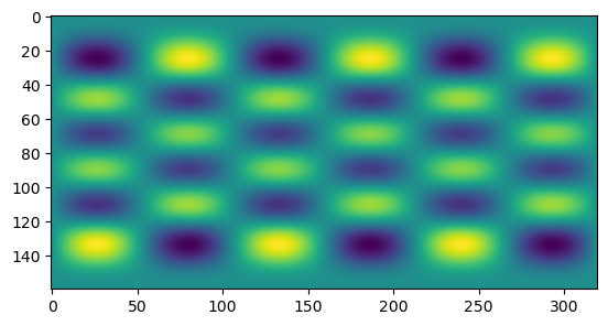
That's it! ecTrans is quite an intimidating package at first, but almost all the complexity comes from the parallel aspects. For performing a simple serial spectral transform it's quite simple.

Performing a direct spectral transform

To close the loop, we can now add a direct transform back to spectral space. Let's do that into a new spectral field array, and compare it with the original. Hopefully they will be equivalent within a tolerable error margin. Declare another allocatable variable SPECTRAL_FIELD_2 and allocate it the same way as with SPECTRAL_FIELD. Now call DIR_TRANS like this:

CALL DIR_TRANS(PGP=GRID_POINT_FIELD, PSPSCALAR=SPECTRAL_FIELD_2)

and compute the error between the first and second spectral field arrays:

WRITE(*,*) "Error = ", NORM2(SPECTRAL_FIELD_2 - SPECTRAL_FIELD)

You should get an error of $O(10^{-7})$ which is roughly the machine epsilon of the single-precision float type $2^{-23} \approx 10^{-7}$. This concludes the demonstration.