Design » Grid

Introduction

In the NWP and climate modelling community (as opposed to, for instance, the engineering community) the grid is often a fixed property for a model. One of Atlas’ goals is to provide a catalogue of a variety of global and regional grids defined by the World Meteorological Organisation in order to support multiple models and model inter-comparison initiatives.

There exist three main categories of grids in terms of functionality that Atlas can currently represent: unstructured grids, regular grids, and reduced grids.

Unstructured grids describe an arbitrary number of points in no particular order. The x- and y-coordinates of the points cannot be computed with certain mathematical formulations, and thus have to be specified individually for each point (e.g. refFigure{unstructured-grid}).

Regular grids on the other hand make the assumption that points are aligned in both x- and y-direction (e.g. refFigure{regular-grid}). Grid point coordinates can then be derived by two independent indices (i, j) associated to the x- and y- direction, respectively.

For reduced grids, lines of constant y or so called parallels may however have a different amount of gridpoints along the x-direction (refFigure{structured-grid} and refFigure{structured-O16-grid}). Reduced grids are a common type of grid employed in global weather and climate models to reduce the number of points towards the poles in order to achieve a quasi-uniform resolution on the sphere.

For both regular and reduced grids, no assumptions are made on the spacing between the parallels in the y direction. The points in x-direction on every parallel are assumed to be equispaced.

Atlas provides grid construction facilities based on a configuration object of the type class{Config} to create global grids or regional grids. For most global grids, this configuration object can also be inferred from a simple string identifier or emph{name} containing one or more numbers representing the grid resolution. Commonly used global grids that can currently be accessed through such name are:

regular longitude-latitude grid (name: L<NLON>x<NLAT> or L<N>);
shifted longitude-latitude grid (name: S<NLON>x<NLAT> or S<N>);
regular Gaussian grid (name: F<N>);
classic reduced Gaussian grid (name: N<N>);
octahedral reduced Gaussian grid (name: O<N>).

In the identifiers shown in this list, <NLON> stands for the number of longitudes, <NLAT> for the number of latitudes, and <N> for the number of parallels between the North Pole and equator (interval ). These grids will be explained in more detail following sections.

Projection

In order to support regional grids for the Limited Area Modelling (LAM) community, projections are often needed that transform so called grid coordinates (x, y) to geographic coordinates (longitude,latitude). For regional grids, the grid coordinates are often defined in meters on a regular grid, as is the case for e.g. a Lambert conformal conic projection and a Mercator projection. Another example projection that is also applicable to a global grid is the Schmidt projection.

In Atlas, the projection is embodied by a Projection class, illustrated in refFigure{grid-Projection}. It wraps an abstract polymorphic class{ProjectionImplementation} class with currently 6 concrete implementations:

LonLatProjection ( type: lonlat, units: degrees, identity )
RotatedLonLatProjection ( type: rotated_lonlat, units: degrees )
SchmidtProjection ( type: schmidt, units: degrees )
RotatedSchmidtProjection ( type: rotated_schmidt, units: degrees )
MercatorProjection ( type: mercator, units: meters, regional )
RotatedMercatorProjection ( type: rotated_mercator, units: meters, regional )
LambertAzimuthalEqualAreaProjection ( type: lambert_azimuthal_equal_area, units: meters, regional )
LambertConformalConicProjection ( type: lambert_conformal_conic, units: meters, regional )

The Projection furthermore exposes functions to convert xy coordinates to lonlat coordinates and its inverse.

For more information about each concrete projection implementation, refer to ESCAPE deliverable report D4.4 cite{D4.4}.

Domain

In this section, the Domain class is introduced (refFigure{grid-Domain}). Its purpose is only useful for non-global grids, and can be used to detect if any coordinate (x, y) is contained within the domain that envelops the grid. The design follows the same principle as the Projection: the Domain class wraps an abstract polymorphic DomainImplementation class with currently 3 concrete implementations:

RectangularDomain ( type: rectangular )
ZonalBandDomain ( type: zonal_band, units: degrees )
GlobalDomain ( type: global, units: degrees )

The domain has no knowledge of any grid projection. Therefore the points that can be tested to be contained inside the domain must be provided in grid coordinates (x, y), and not in geographical coordinates (lon, lat).

The RectangularDomain domain defines a rectangular region defined by 4 values: , , , . These values must be defined in units that correspond to the used grid projection. The ZonalBandDomain domain assumes that the units of x and y are in degrees, and that the domain is periodic in the x-direction. Therefore, to test if a point is contained within this domain only requires to check if the point’s y coordinate lies in the interval . The GlobalDomain domain, like the ZonalBandDomain domain assumes units in degrees, and always evaluates that any point is contained within.

Supported Grid types

Atlas provides a basic Grid class that can embody any unstructured, regular or reduced grid. The Grid class is a wrapper to an abstract polymorphic class{GridImplementation} class with 2 concrete implementations: class{Unstructured} and class{Structured}. The class{Unstructured} implementation holds a list of (x, y) coordinates (one pair for each grid point). The Structured implementation follows the assumption of a reduced grid. It holds a list of y-coordinates (one value for each grid parallel), a list of number of points for each parallel, and a list of x-intervals (one pair for each parallel) in which the points for the parallel are uniformly distributed. With the Structured implementation, both reduced and regular grids can be represented, as regular grids can also be interpreted as a special case of a reduced grid (where every parallel contains the same number of points).

Following code snippets shows how to construct any grid from either a configuration object or a name, both in C++ and Fortran.

Example on construction of grids

C++ example:

Config F16_config;
F16_config.set( "type", "regular_gaussian" );
F16_config.set( "N", 16 );

Grid F16( F16_config );   // regular Gaussian grid (F16)
Grid N16( "N16" );        // classic reduced Gaussian (N16)

Fortran example:

type(atlas_Grid)   :: F16, N16
type(atlas_Config) :: F16_config
...
F16_config = atlas_Config()
call F16_config%set( "type", "regular_gaussian" )
call F16_config%set( "N", 16 )

F16 = atlas_Grid( F16_config )  ! regular Gaussian grid (F16)
N16 = atlas_Grid( "N16" )       ! classic reduced Gaussian grid (N16)

Even though the configuration object (F16_config) is here constructed programatically, it may also be imported through a JSON string or file. The regular Gaussian grid could also be constructed through a name F16. Similarly the classic reduced Gaussian grid could also be constructed through a config object with the type classic_gaussian.

refFigure{grid-Grid} illustrates the Grid class implementation. It shows that the Grid class can return instances of the Domain class and the Projection class.

Because this basic Grid class can make no assumptions on whether it wraps a class{Structured} or a class{Unstructured} concrete implementation, it can only expose an interface for the most general type of grids: the class{Unstructured} approach. This means that we can find out the number of grid points with the Grid::size() function, and that we can iterate over all points, assuming no particular order. The following C++ code shows how to iterate over all points, and use the projection to get longitude-latitude coordinates.

// Iterating over all points of a octahedral reduced Gaussian grid O1280

Grid grid( "O1280" );
Log::info() << "The grid contains " << grid.size() << " points. \n";
for( PointXY p, grid ) {
    Log::info() << "xy: " << p << "\n";
    double x = p.x();
    double y = p.y();

    PointLonLat pll = grid.projection().lonlat(p);
    Log::info() << "lonlat: " << pll << "\n";
    double lon = pll.lon();
    double lat = pll.lat();
}

In above C++ code we used the projection to compute the longitude and latitude coordinates. For the used octahedral Gaussian grid however, the projection is of the lonlat type by construction, meaning that x and y are already equivalent to lon and lat respectively. The second part in the for loop was thus not necessary for this particular grid.

The basic Grid class shown in refFigure{grid-Grid} also exposes a function Grid::uid() which returns a string which is guaranteed to be unique for every possible grid. This includes differences in projections and domains as well.

To be able to expose more structure or properties present in the grid, a number of grid interpretation classes are available, that also wrap the used class{GridImplementation}, but try to cast it to the class{Structured} implementation if necessary. Currently available interpretations classes are:

UnstructuredGrid: The grid is unstructured and cannot be interpreted as structured.
StructuredGrid: The grid may be regular or reduced.
RegularGrid: The grid is regular.
ReducedGrid: The grid is reduced, and not regular.
GaussianGrid: The grid may be a global regular or reduced Gaussian grid.
RegularGaussianGrid: The grid is a global regular Gaussian grid.
ReducedGaussianGrid: The grid is a global reduced Gaussian grid, and emph{not} a regular grid.
RegularLonLatGrid: The grid is a global regular longitude-latitude grid.
RegularPeriodicGrid: The grid is a periodic (in x) regular grid.
RegularRegionalGrid: The grid is a regional non-periodic regular grid, and can have any projection.

Note that there is no use case for interpreting a grid as e.g. octahedral reduced Gaussian or classic reduced Gaussian, as it does not bring any benefit over the ReducedGaussianGrid interpretation class.

Just like the basic Grid class, these interpretation classes have a function valid(). Rather than throwing errors or aborting the program if the constraints listed above are not satisfied, the user has to call the valid() function to assert the interpretation is possible. refFigure{grid-Tree} illustrates the above list schematically. Arrows indicate a can be interpreted by relationship.

For a NWP model, you can usually safely assume the grid interpretations as the model can usually only work with a certain type of grid. ECMWF’s IFS-model for instance, can assume that all used grids can be interpreted by the GaussianGrid class, whereas a LAM-model could e.g. assume the RegularRegionalGrid interpretation.

UnstructuredGrid

The UnstructuredGrid interpretation class constrains the grid implementation to be class{Unstructured}. No assumption on any form of structure can be made. Also no assumption on the domain nor the projection used is made.

refFigure{grid-UnstructuredGrid} shows the UML class diagram of the StructuredGrid. The first two constructors listed effectively create a new grid, whereas the third constructor accepts any existing grid, and reinterprets it instead. No copy or extra storage is then introduced, since the wrapped GridImplementation is a reference counted pointer (a.k.a. shared_ptr), of which the reference count is increased and decreased upon UnstructuredGrid construction and destruction respectively.

An UnstructuredGrid exposes two extra functions UnstructuredGrid::xy(n) and UnstructuredGrid::lonlat(n). The first function gives random access to the (x, y) coordinates of grid point n. The second function is a convenience function that internally uses the grid Projection to project the grid coordinates xy(i, j) to geographic coordinates.

StructuredGrid

The StructuredGrid interpretation class constrains the grid implementation to be class{Structured}. The grid may be regular or reduced. It makes no assumptions on whether the domain is global, periodic, or regional, or whether any projection is used. Almost any grid with some form of structure in a single area can therefore be interpreted by this class.

refFigure{grid-StructuredGrid} shows the UML class diagram of the StructuredGrid. The first two constructors listed effectively create a new grid, whereas the third constructor accepts any Grid, and reinterprets it instead if possible. No copy or extra storage is then introduced, since the wrapped class{GridImplementation} is a reference counted pointer (a.k.a. shared_ptr), of which the reference count is increased and decreased upon StructuredGrid construction and destruction respectively.

With the information that the grid can only be reduced or regular, new accessor functions can be exposed to access grid points more effectively through indices (i, j). The only functions that can be guaranteed to apply for both regular and reduced grids, are the ones that assume a reduced grid. This means that the x coordinate and the number of points on a parallel depend on the parallel itself, denoted by index j. For convenience, a function lonlat(i, j) is available that internally uses the grid Projection to project the grid coordinates xy(i, j) to geographic coordinates.

RegularGrid

A RegularGrid is a specialisation of a StructuredGrid by further constraining that the number of points on every parallel is equal. In other words, points are now also aligned in y direction. The grid then forms a Cartesian coordinate system.

With this information, access to the x coordinate of a point is now independent of the index j, and only depends on the index i. The relevant functions that can be adapted now are RegularGrid::nx() and RegularGrid::x(i). Using these functions can possibly increase the performance of algorithms.

ReducedGrid

A ReducedGrid is, unlike the RegularGrid, not a specialisation of the StructuredGrid in terms of functionality, but it does add the constraint that the grid is only valid when it is not regular. refFigure{grid-ReducedGrid} shows the class diagram for this type of grid.

GaussianGrid

A GaussianGrid is a StructuredGrid with the additional constraint that the grid is globally defined with an even number of parallels that follow the roots of a Legendre polynomial in the interval cite{Hortal1991}. This class exposes an additional function GaussianGrid::N(), which is the so called Gaussian number, equivalent to the number of parallels between the North Pole and the equator. The x-coordinate of each first point of a parallel starts at (Greenwich meridian). refFigure{grid-GaussianGrid} shows the class diagram for the GaussianGrid.

RegularGaussianGrid

A RegularGaussianGrid combines the properties of a RegularGrid and a GaussianGrid. It can be defined by a single number N (the Gaussian number). The number of points in x- and y-direction are by convention begin{align*} nx &= 4 N \ ny &= 2 N end{align*} refFigure{grid-RegularGaussianGrid} shows the class diagram for the RegularGaussianGrid. begin{figure}[htb!] centering includegraphics[scale=0.5]{figures/grid/RegularGaussianGrid.pdf} caption{UML class diagram for the RegularGaussianGrid class } label{figure:grid-RegularGaussianGrid} end{figure} As can be seen in the class diagram, an additional constructor is available, taking only this Gaussian number N, so that it is easy to create grids of this type. These grids can also be created through the constructor taking the name F<N>, with <N> the Gaussian number N.

ReducedGaussianGrid

A ReducedGaussianGrid combines the properties of a ReducedGrid and a GaussianGrid. A single number N (the Gaussian number), defines the number of parallels (ny = 2 N), but no assumptions are made on the number of points on each parallel.

refFigure{grid-ReducedGaussianGrid} shows the class diagram for the ReducedGaussianGrid.

As can be seen in the class diagram, an additional constructor is available, taking an array of integer values with size equal to the number of parallels (must be even). The values correspond to the number of points for each parallel. The WMO GRIB standard also refers to this array as PL, and IFS refers to this array as NLOEN. In Atlas it is referred to as the array nx (cfr. the StructuredGrid). The number of parallels ny is inferred by the length of this array, and the Gaussian N number is then ny/2, which is used to define the y-coordinate of the parallels.

Classic reduced Gaussian grids

In practise we tend to use only a small subset of the infinite possible combinations of reduced Gaussian grids for a specific N number. Until around 2016, ECMWF’s IFS-model was using reduced Gaussian grids for which the nx-array was not straightforward to compute. These arrays for all used reduced Gaussian grids were tabulated. We now refer to these grids as classic reduced Gaussian grids, and they can be created through the name N<N>, with <N> the Gaussian number N. Not any value of N is possible because there are only a limited number of such grids created (only the ones used). Atlas can create classic reduced Gaussian grids for values of N in the list [ 16, 24, 32, 48, 64, 80, 96, 128, 160, 200, 256, 320, 400, 512, 576, 640, 800, 1024, 1280, 1600, 2000, 4000, 8000 ].

Octahedral reduced Gaussian grids

Since around 2016, ECMWF’s IFS-model now uses reduced Gaussian grids for which the nx-array can be computed by a simple formula rather than a complex algorithm. These grids are referred to as octahedral reduced Gaussian grids. The nx-array can be computed as follows in C++:\

// Computing the `nx`-array for octahedral reduced Gaussian grids, C++ example,
int jLast = 2*N-1;
for( int j=0; j<N; ++j ) {
  nx[j] = 20 + 4*j;    // Up to equator
  nx[jLast-j] = nx[j]; // Symmetry around equator
}

In order to refer to these grids easily in common language, and to more easily construct these grids using the constructor taking a name, the name O<N> was chosen, with <N> the Gaussian number N, and O referring to octahedral. The term octahedral originates from the inspiration to project a regularly triangulated octahedron to the sphere. Few modifications to the resulting grid were made to make it a suitable reduced Gaussian grid for a spectral transform model cite{malardel2016new}.

RegularLonLatGrid

The RegularLonLatGrid is likely the most commonly used grid on the sphere. It is a global grid regular grid defined in degrees with a uniform distribution both in x- and in y-direction. Atlas supports 4 variants of the RegularLonLatGrid, each with 2 identifier names: begin{itemize} item standard: L<NLON>x<NLAT> or L<N> item shifted: S<NLON>x<NLAT> or S<N> item longitude-shifted: Slon<NLON>x<NLAT> or SLON<N> item latitude-shifted: Slat<NLON>x<NLAT> or SLAT<N> end{itemize} In the identifier names, <NLON> and <NLAT> denote respectively nx and ny of a regular grid. For ease of comparison with the Gaussian grids, these grids can also be named instead with a N number denoting the number of parallels in the interval – between the North Pole and equator by including Pole and excluding equator. The x- and y-increment is then computed as . For each of the grids, all points are defined in the range and . For the emph{standard} case, the first and last parallel are located exactly at respectively the North and South Pole. Usually the number of parallels ny=<NLAT> is odd, so that there is also exactly one parallel on the equator. It is also guaranteed that the first point on each parallel is located on the Greenwich meridian (). In this context, emph{shifted} denotes a shift or displacement of x- and y-coordinates of all points with half increments with respect to the standard (or unshifted) case. In order to achieve the same x- and y-increment as the emph{standard} case, the emph{shifted} case should be constructed with one less parallel. The two remaining cases emph{longitude-shifted} and emph{latitude-shifted} shift only respectively the x or y coordinate of each grid point.

refFigure{grid-RegularLonLatGrid} shows the class diagram for the RegularLonLatGrid. It can be seen that this class exposes 4 functions to query which of the 4 variants is presented.

RegularPeriodicGrid

The RegularPeriodicGrid can be used to assert that the grid is a regular grid with equidistant spacing in x- and y-direction, and with periodicity in the x-direction. The latter enforces an implicit additional constraint that x and y are defined in degrees. refFigure{grid-RegularPeriodicGrid} shows the class diagram for the RegularPeriodicGrid.

RegularRegionalGrid

The RegularRegionalGrid is a grid that asserts that the grid is not global nor periodic. The gridpoints must be equidistant both in x- and y-direction. No restrictions on projections are made. This grid would be the typical use-case grid to use in conjuction with e.g. a Lambert, Mercator, or RotatedLonLat projection. refFigure{grid-RegularRegionalGrid} shows the class diagram for the RegularRegionalGrid.

Construction of grids of this type can be done in various ways through configuration.

Partitioner

Even though the class{Grid} object itself is not distributed in memory as it does not have a large memory footprint, it is necessary for parallel algorithms to divide work over parallel MPI tasks.

There exist various strategies in how to partition a grid, where each strategy may offer different advantages, depending on the grid and numerical algorithms to be used.

Atlas implements a grid class{Partitioner} class, that given a grid, partitions the grid and creates a class{Distribution} object that describes for each grid point which partition it belongs to. refFigure{grid-Partitioner} illustrates the UML class diagram for the class{Partitioner} class. Following a similar design philosophy as before, the class{Partitioner} class wraps an abstract polymorphic class{PartitionerImplementation} object. refFigure{grid-Distribution} illustrates the UML class diagram for the class{Distribution} class.

Currently there are 3 concrete implementations of the class{PartitionerImplementation}:

Checkerboard ( type: checkerboard ) – Partitions a grid in regular zones
EqualRegions ( type: equal_regions ) – Partitions a grid in equal regions, reminiscent of a disco ball.
MatchingMesh ( type: matching_mesh ) – Partitions a grid such that grid points following the domain decomposition of an existing mesh which may be based on a different grid.
MatchingFunctionSpace ( type: matching_functionspace ) – Partitions a grid such that grid points following the domain decomposition of an existing functionspace which may be based on a different grid.

The class{Checkerboard} and class{EqualRegions} implementations can be created from a configuration object only. The class{MatchingMesh} implementation requires a further mesh argument to its constructor. For this reason, a class{MatchingMeshPartitioner} class exists whose only purpose is that it knows how to construct its related class{MatchingMesh} implementation with the extra mesh argument.

Checkerboard Partitioner

For regular grids, such as the one depicted in refFigure{regular-grid}, a logical domain decomposition would be a checkerboard. The grid is then divided as well as possible into approximate rectangular zones in Cartesian grid coordinates (x, y) with an equal number of grid points. An example of this partitioning algorithm is shown in refFigure{grid-Checkerboard-example}.

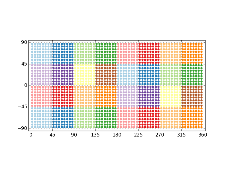
Example class{Checkerboard} partitioning of a shifted regular longitude-latitude grid `S64x32` in 32 partitions.

EqualRegions Partitioner

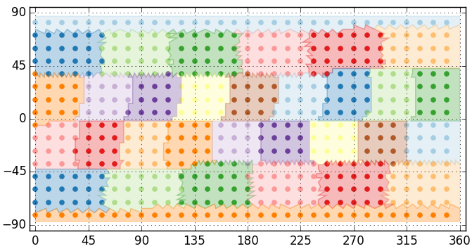
For reduced grids as the ones shown in refFigure{structured-grid} and refFigure{structured-O16-grid} or for uniformly distributed unstructured grids, an equal regions domain decomposition is more advantageous cite{deconinck2016accelerating,leopardi2006partition,Mozdzynski2007}. The equal regions partitioning algorithm divides a two-dimensional grid of the sphere (i.e. representing a planet) into bands from the North pole to the South pole. These bands are oriented in zonal directions and each band is then split further into regions containing equal number of grid points. The only exceptions are the bands containing the North or South Pole, that are not subdivided into regions but constitute North and South polar caps.

An example of this partitioning algorithm is shown in refFigure{grid-EqualRegions-example}

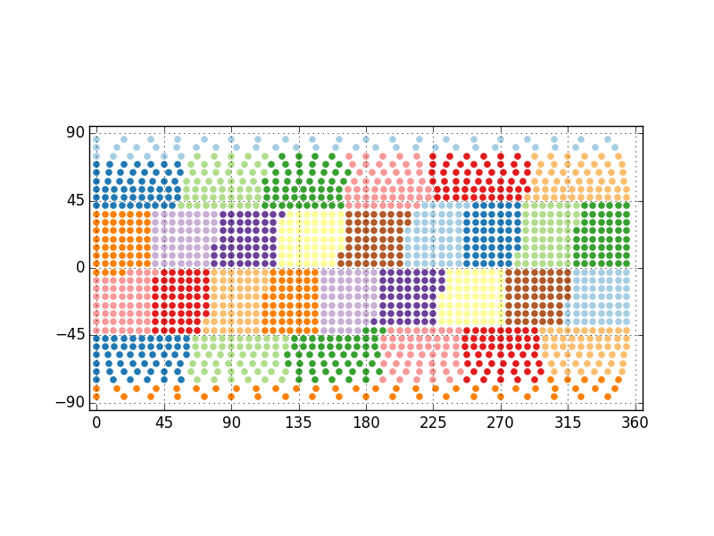
Example class{EqualRegions} partitioning of a idx{N16} classic reduced Gaussian grid in 32 partitions.

MatchingMesh Partitioner

The class{MatchingMeshPartitioner} allows to create a class{Distribution} for a grid such that the grid points follows the domain decomposition of an existing mesh (described in detail in refSection{mesh}). This partitioning strategy is particularly useful when grid points of a partition should be contained within a mesh partition present on the same MPI task to avoid parallel communication during coupling or interpolation algorithms. Note that there is no guarantee of any load-balance here for the partitioned grid. refFigure{grid-MatchingMeshPartitioner-example} shows an example application of the class{MatchingMeshPartitioner}.

Example partitioning in 32 parts of a F8 rectangular Gaussian grid (solid dots) using the domain decomposition of an existing meshed N24 classic reduced Gaussian grid. Each domain is shaded and surrounded by a solid line. The jagged lines of the existing N24 mesh subdomains are contours of its elements.